 |  |
The following treats the problem of computing distances and shortest geodesics (the generalization of straight lines to general manifolds) on polyhedral metrics, given only the intrinsic surface in the form of a graph that represents the 1-skeleton of the polyhedron. That is, no reference is made to any embedding in 3D. This is a necessary step towards calculating electron repulsion on carbon manifold directly from their graphs, without the need for an expensive optimization step to find their 3D geometries.
The algorithm I derive is specialized to simplical metrics, i.e., surfaces with faces that are equilateral triangles. However, by the method we describe in Wirz, Schwerdtfeger, and Avery 2017, Naming Polyhedra by General Face-Spirals, this can be extended through a leapfrog transformation to general polyhedral metrics.
The code is included in our open source fullerene analysis program Fullerene, and used in the experimental methods for direct embedding calculations, as well as the pilot DFT calculations directly on the manifold. However, the work is not yet published: A paper is in preparation, and I ask the grant referees to not share any of this work yet.
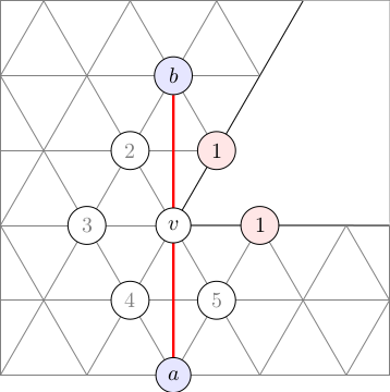
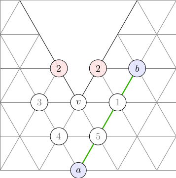
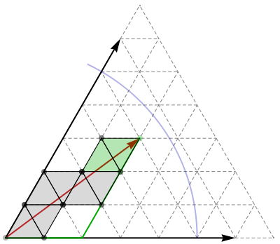
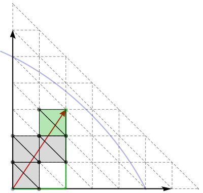
Unlike the case of a sphere, there are in general many geodesics connecting any two points, and three points do not define a unique triangle. The figure here shows two straight lines of different lengths that connect the same two points.
Figure 1 shows two geodesics lines of different lengths that connect the same two points, corresponding to two different cuts, each unfolded into the Eisenstein plane as a straight line. One goes through $v$, the other goes around it, but is shorter.
| |
Generally, the number of geodesics that connect any two points on a polyhedral metric surface grows exponentially in the number of cone-points, i.e., the vertices that induce its Gaussian curvature. For simplical surfaces (that have equilateral triangle faces), these are the vertices of degree ≠ 6 (dually, the non-hexagon faces for cubic graph surfaces). Further, the bumpy, curved surfaces do not admit any global, isometric 2D-coordinate system, i.e., we cannot find a single, flat 2D coordinate system for the whole bumpy, curved surface, making geometry difficult.
However, pairs of adjacent simplices share a Cartesian coordinate system. Outside the pair, the coordinate system is invalid (and geometric operations will yield gibberish if neighbouring a cone point), but inside such a pair, lengths and angles are "flat", and we can calculate them as we are used to from Cartesian coordinate systems.
 |
 |
The algorithm below exploits this fact for calculating geodesics through overlapping patches of Cartesian coordinate systems.
The algorithm rests on a lemma stating that shortest geodesics can be understood to be piecewise linear in the sense that the sequence of faces that a shortest geodesic passes through can be cut out and laid out flat in the Eisenstein plane (isometrically, i.e., without changing the surface distances). The geodesic can then be drawn as a finite sequence of straight lines, each never crossing through a cone point singularity, but possibly ending at one. In addition, for convex polyhedral metrics (such as those of fullerene surfaces), shortest geodesics consist of a single "straight line". Note, however, that the concept of "straight line" is not straight forward, as illustrated in Figure 1.
More precisely, geodesics are composed of simple paths, defined as follows:
Definition, Simple Path:
A simple path is one that does not pass through
cone points (vertices with degree ≠ 6) except at its end points.
Lemma 1: Shortest geodesics are piecewise simple.
Proof.Lemma 2: Shortest geodesics never pass through a positive-curvature cone-points.
Proof.Lemma 3: Any segment of a shortest geodesics contained within any Cartesian coordinate system patch will be a straight line in this coordinate system.
Proof.Corollary: Shortest geodesics on convex polyhedral metrics are simple.
Convex polyhedral metrics are characterized by having no non-convex cone-points, i.e., vertices with degree > 6, i.e., all cone-points are convex. By Lemmas 1 and 2 it follows that a shortest geodesics on a convex polyhedral metric must be simple.Thus, we can solve the general problem by solving the simple-path connection problem. For convex polyhedral metrics, this is the end, yielding shortest geodesics and distances. Non-convex metrics require one extra step: computing shortest paths in the "shortest simple-paths" connection graph (weighted by the shortest simple path lengths). In my implementation, I simply compute all-pairs-shortest-paths using matrix-multiplication in the min/+-semiring, a standard method for APSP in dense weighted graphs, but any other standard method can be used.
Because shortest geodesics are piecewise simple, we can reduce the problem to that of finding shortest simple paths, and combining these to form the shortest geodesics.
The following two observations are each somewhat trivial, but together they point towards an algorithm that efficiently finds the shortest simple paths:
Observation 1: The surface distance $d(u,v)$ between two vertices $u$ and $v$ is bounded from above by $D(u,v)$, the graph-distance (along edges) between $u$ and $v$.
Observation 2: Let $M = \max_v D(u,v)$ be the largest graph distance from $u$. Then a shortest simple path $u$—$v$ can be represented as a straight line, drawn on a triangle strip in the Eisenstein plane. The path-segment in the overlapping coordinate systems between successive triangle pairs uniquely determines the line's continuation in the next coordinate system. When $u$ is given Eistenstein coordinate $(0,0)$, then $v$ has coordinates $(a,b)$, where $|(a,b)| = \sqrt{a^2+ab+b^2} \le M$.
Observation 3: Conversely, if we can "draw" an Eisenstein line $(0,0)$—$(a,b)$ from vertex $u$, and by "drawing" it reach vertex $v$, then $d(u,v)^2 \le a^2 + ab + b^2$.
Observation 4: We can "draw" an Eisenstein line to $(a,b)$ relative to $u$ and find the vertex $v$ at its endpoint by successively laying down the triangles in the Eisenstein plane, each time the line crosses an edge into a new face. The result will be a straight line drawn on the laid down triangles in the Eisenstein plane (but curved in an isometric 3D embedding of the surface).
From this, we can formulate an outline of an algorithm:
|
|
 |
↦ |  |
matrix<int> Triangulation::convex_square_surface_distances() const
{
  matrix<int> H = matrix<int>(N,N,all_pairs_shortest_paths());
  int M = *max_element(H.begin(),H.end());      // M is upper bound to path length

  for(int i=0;i<H.size();i++) H[i] *= H[i]; // Work with square distances, so that all distances are integers.

  for(node_t u=0;u<N;u++)
    for(int i=0;i<neighbours[u].size();i++){

      // Note: All Eisenstein numbers of the form (a,0) or (0,b) yield same lengths
      //       as graph distance, and are hence covered by initial step. So start from 1.
      //       M is upper bound for distance, so only need to do a^2+ab+b^2 strictly less than M.
      for(int a=1; a<M;a++)
        for(int b=1; a*a + a*b + b*b < M*M; b++){
          // Check: if(gcd(a,b) != 1) continue.
          const node_t v = end_of_the_line(u,i,a,b);

          H(u,v) = min(H(u,v), a*a + a*b + b*b);
        }
    }
  return H;
}
// Given start node u0 and adjacent face F_i, lay down triangles along the the straight
// line to Eisenstein number (a,b), and report the endpoint-node.
//
// Assumes a,b >= 1.
node_t Triangulation::end_of_the_line(node_t u0, int i, int a, int b) const
{
  node_t q,r,s,t;                // Current square

  auto go_north = [&](){
    const node_t S(s), T(t); // From old square
    q = S; r = T; s = next(S,T); t = next(s,r);
  };

  auto go_east = [&](){
    const node_t R(r), T(t); // From old square
    q = R; s = T; r = next(s,q); t = next(s,r);
  };

  // Square one
  q = u0;                       // (0,0)
  r = neighbours[u0][i];        // (1,0)
  s = next(q,r);                // (0,1)
  t = next(s,r);                // (1,1)

  if(a==1 && b==1) return t;

  vector<int> runlengths = draw_path(max(a,b), min(a,b));

  for(int i=0;i<runlengths.size();i++){
    int L = runlengths[i];

    if(a>=b){                        // a is major axis
      for(int j=0;j<L-1;j++)    go_east();
      if(i+1<runlengths.size()) go_north();
    } else {                        // b is major axis
      for(int j=0;j<L-1;j++)    go_north();

      if(i+1<runlengths.size()) go_east();
    }
  }

  return t;                        // End node is upper right corner.
}
vector<int> draw_path(int major, int minor)
{
  int slope = major/minor, slope_remainder = major%minor, slope_accumulator = 0;

  vector<int> paths(minor+1,0), runs(minor);

  for(int i=0; i<minor; i++){
    slope_accumulator += slope_remainder;

    paths[i+1] = paths[i] + slope + (slope_accumulator != 0);

    if((i+1<minor) && (slope_accumulator >= minor || slope_remainder == 0)){
      paths[i+1]++;
      slope_accumulator %= minor;
    }

    runs[i]    = paths[i+1]-paths[i];
  }
  return runs;
}
matrix<double> Triangulation::surface_distances() const
{
  matrix<double> H(convex_square_surface_distances());
  for(int i=0;i<N*N;i++) H[i] = sqrt(H[i]);

  bool nonconvex = false;
  for(node_t u=0;u<N;u++) if(neighbours[u].size() > 6) nonconvex = true;

  if(nonconvex) return H.APSP();
  else return H;
}
  static matrix minplus_multiply(const matrix& A, const matrix& B, const T& infty_value = USHRT_MAX)
  {
    assert(A.n == B.m);
    matrix C(A.m,B.n);

    for(int i=0;i<A.m;i++)
      for(int j=0;j<B.n;j++){
	T x = infty_value;
	for(int k=0;k<A.n;k++) x = min(x, T(A[i*A.n+k]+B[k*B.n+j]));
	x = min(x,infty_value);
	C[i*C.n+j] = x;
      }
    return C;
  }

  matrix APSP() const {
    int count = ceil(log2(m));
    matrix A(*this);
    for(int i=0;i<count;i++) A = minplus_multiply(A,A);

    return A;
  }