Applied Statistics - Week 3
Monday the 3rd - Friday the 7th of December 2018
ERDA shared link to full week material:
G5MICBv1j0
ERDA shared link to solution examples:
DnVCa3Nwi5
The following is a description of what we will go through during this
week of the course. The chapter references and computer exercises are
considered read, understood, and solved by the beginning of the
following class, where I'll shortly go through the exercise
solution.
General notes, links, and comments:
Monday:
Experiments for project: (Group B)
We will be working on the experiments for
Project in First Lab.
This project should be handed in (PDF by mail to me) by 22:00 on Sunday the
16th of December 2018 (please, don't sit up all night!).
I would be happy, if you would give the file the logical name
"Project_GroupX_Name1Name2Name3Name4Name5.pdf", where NameX is the
first name of the group members.
Lectures and exercises: (Group A)
Real data almost never follows theoretical PDFs, as the real world
contains dirty wires, unknown biases, and mismeasurements. We will
devote the day to discussion of real data analysis and systematic
errors, and apply this to our "Table Measurements" from Aud. A.
Reading:
Barlow, chapter 4.4
Chauvenet's
Criterion on Wikipedia
Lecture(s):
Systematic Uncertainties (given by Jason):
Systematic Errors
Computer Exercise(s):
TableMeasurements:
TableMeasurement.py,
data_TableMeasurements2009.txt
data_TableMeasurements2010.txt
data_TableMeasurements2011.txt
data_TableMeasurements2012.txt
data_TableMeasurements2013.txt
data_TableMeasurements2014.txt
data_TableMeasurements2015.txt
data_TableMeasurements2016.txt
data_TableMeasurements2017.txt
data_TableMeasurements2018.txt
In addition, the 2018 data exists in an expanded format, where two
columns are added: Gender (M/F - sorry, no third gender option, except
blank) and if the speed was done with pleanty of time (i.e. in Week0)
or at high pace (Monday the 19th).
If you managed to get a (good?) result on the "standard" problem, you
can consider if the hurried measurements are worse or more faulty than
the slower ones, and/or if there is any difference between men and
women in the measurements:
data_TableMeasurements2018_WithGenderSpeedInfo.txt
Tuesday:
We will consider Monte Carlo Techniques, which is a ubiquitious
tool in statistics. The central point is to be able to generate
random numbers according to any given distribution, and subsequently use
this.
Reading:
Glen Cowan: Chapter 3.
Wiki transformation method.
Wiki Hit-and-Miss (Von Neumann) method.
Particle
Data Group (PDG) note on Monte Carlo generators (optional - extends GC chapter 3).
Lecture(s):
Monte Carlo methods.
Computer Exercise(s):
Making Random Numbers according to any distribution: MakingRandomNumbers.ipynb
Transformation vs. HitAndMiss (Reject/Accept) method: TransHitMiss.ipynb
Friday:
The main theme will again be the Likelihood function, and how
to use it when fitting data. This time the example is more advanced
and a classic fitting case - some background with a possible Gaussian
peak on it.
In addition, I'll be lecturing on types of data and ways of plotting,
and we'll shortly discuss Simpson's Paradox, which we jumped over a
bit last week!
Reading:
Barlow, chapter 5.3 to 5.7 (but not 5.5 and the proofs).
Lecture(s):
Types of data and ways of plotting
Simpson's Paradox
Computer Exercise(s):
ExampleLikelihoodFit.ipynb: ExampleLikelihoodFit.ipynb
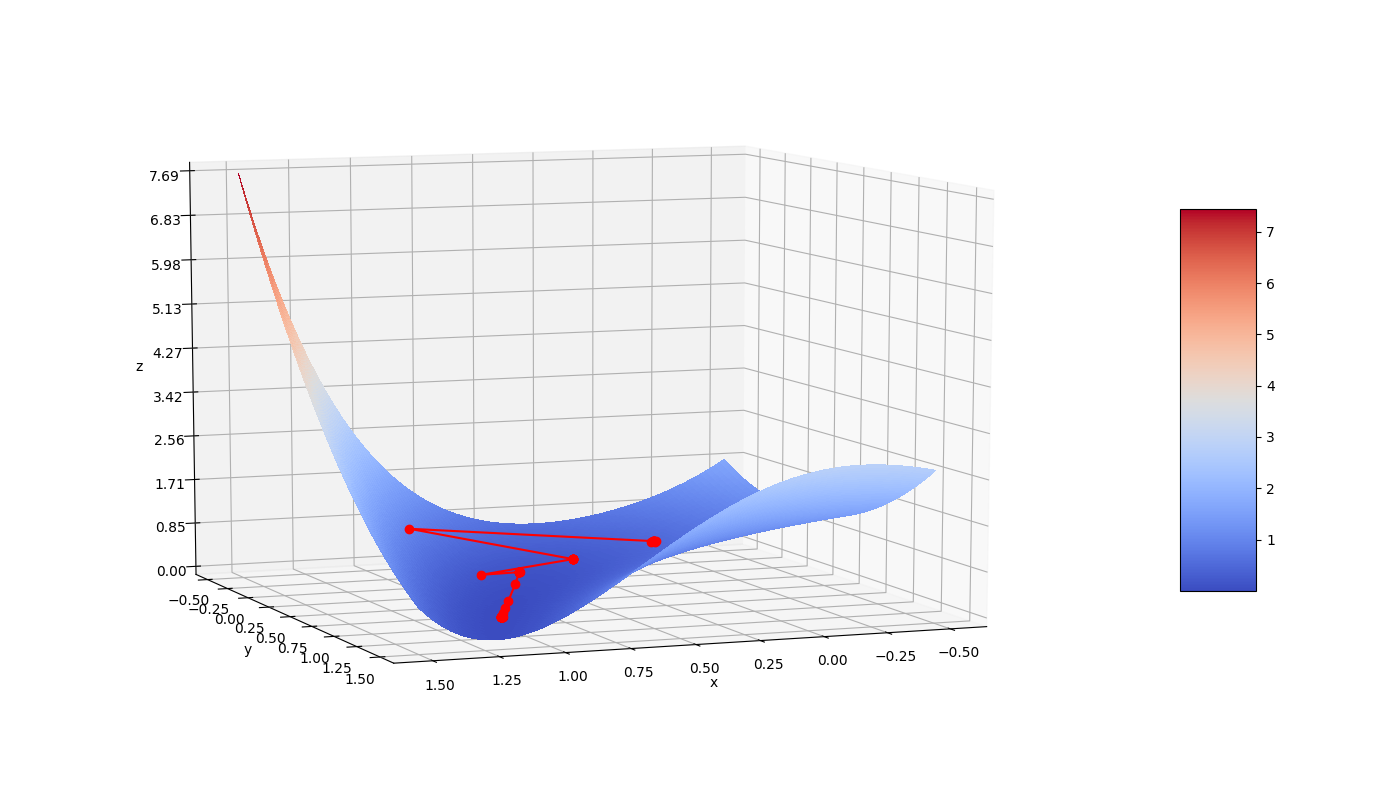
TrackMinimizer.ipynb: TrackMinimizer_ForIllustration.ipynb
which produces Fig_TrackMinuit.png
Simpson's paradox: Simpsons_Paradox.ipynb
Last updated: 3rd of December 2018.