Applied Statistics - Project 1
Project description:It is the year 1679, and Hooke is (following a suggestion from Newton) trying to prove the rotation of Earth by the Coriolis force on falling bodies. Your team has an other (better?) idea, namely to measure the gravitational pull on Earth at different latitudes.
However, to obtain the necessary funding to travel North and South and repeat a measurement of g near the poles and equator, you have to prove that you can do it with the necessary precision. The size of the effect is somewhere around 0.5%, and you want to prove the difference with 5 sigma certainty, which thus requires sub-per-mille precision.
Your mission - and you have little choice, but to accept it - is to take up the challenge of making these measurements and proving that at least one of your two experimental setups has the required/desired precision...
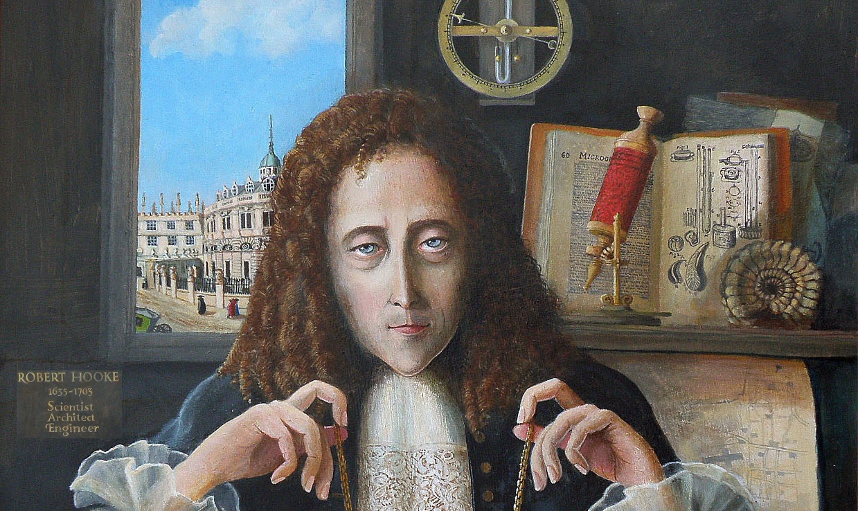
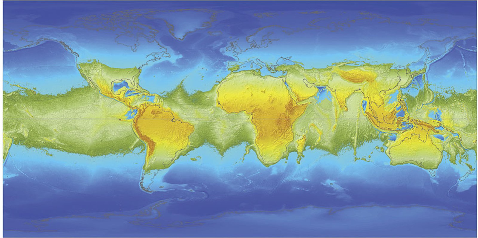
Left: Robert Hooke (1655-1705), Right: The distribution of land and ocean, if Earth's rotation stopped!
Experiments:
The two experiments are classic experiments, and you have almost surely done these before. However, now the aim is learing how to extract, minimize and propagate uncertainties to get a value (in fact two values) for the gravitational acceleration, g, which have as small an uncertainty as possible, but still being consistent with the "true" value (i.e. more precise measurements).
The two experiments are:
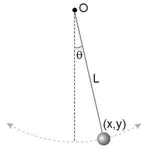
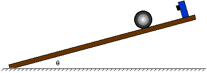
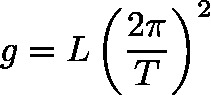
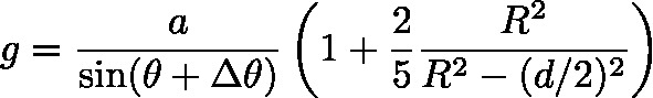
Left: Pendulum experiment with associated formula for g. Right: Ball on incline experiment with associated formula for g.
Suggestions for initial macros:
The following two macros are suggestions for a place to start data analysis. They run on the datasets provided, which should look a bit what you will get!
data_Alice_pendulum14m_25measurements.dat, data_Bob_pendulum14m_25measurements.dat
data_NormDir_MedBall1.txt, data_RevDir_MedBall1.txt
For the pendulum experiment, I suggest copying the analysis macro, and "empty" it, such that you can try to (re-)produce it yourself. Also, for illustrating the period measurement, you may let yourself be inspired by this figure.
Measurements to make:
Below is a list of measurements to make, all of which should of course have well determined uncertainties. Make sure that you report all the "raw" measurements you performed (i.e. for each group or group member), possibly with uncertainty, if one was available. Otherwise, you obtain the uncertainty from the RMS of the typically four independent (make sure they are!) measurements. Typically, all members of the group should do the measurements, and try to read lengths off to 1/2 - 1/10 millimeter.
And finally, you should of course combine your measurements to one value of g for each setup and compare the two both in value and precision.
Writing up results:
The project should be written in Physical Review Letter style (or something close to it, if you don't like Latex) thus not more than 3-4 pages! The aim should be to answer the questions above also given on page two of the introduction slides. You do not need to describe the experiments themselves (assume the reader is a fellow student, who has also done the experiments), but of course all measurements, details and results should be described, such that the reader can follow (i.e. calculate themselves) your results fully and reproduce what you have done.
Below you can find the files needed (works with pdftex as well, except for the figures, which needs to be converted into .pdf or .png):
For each of the two results, I would like to see a table with the errors from each of the variables listed. So for each variable used in determining g, list their value, their uncertainty, and their impact on g (i.e. if they were the only uncertainty on g, how large would it then be), so that one can compare source of error. An example in LaTeX can be found in the PRL template above.
Additional information on the evaluation points (and a challenge) can be found here.
The group should send the project by mail in PDF format to me by Thursday the 7th of December, 22:00.
I would be happy, if you would give the file the logical name "Project1_GroupX_Name1Name2Name3Name4Name5.pdf", where NameX is the first name of the group members.
In addition, we would like each person to submit their timing resolution and residuals, thanks.
If you are in doubt about what we are asking for, then the timing resolution is the RMS of your residuals, i.e. one number (for example 0.078 s), while the residuals are many (15-50 or so) numbers (for example 0.045, 0.083, 0.062, etc.).
The following is the Project1 groups.
Notes:
For measuring time to (better than) 1/100 of a second with lap time and the option of saving the result to a file on your computer, please use the following Python stop watch script: stopwatch.py.
Comments:
Enjoy, have fun, and throw yourself boldly at the data.
Last updated: 24th of November 2017.